Data Table
Table 1 includes a sample of the data prior to any modifications for analysis. Each row contains each measured value from a specific date and location of sampling. Variables missing >90% of observations, or where >90% of the values are below the machine detection limit were removed. Any remaining values below the level of detection were entered into this spreadsheet as 0 concentration.
A small number of MeHg and Hg concentrations were removed due to issues identified during data quality control checks, so a RandomForest model was used to infer the concentrations until samples can be re-analysed.
One dam's water chemistry results indicated that is received primarily groundwater rather than peatland water, so was removed from the analysis as an outlier.
Table 2. A sample of the data table used for the analyses. A total of 36 water chemistry variables are reported in this data sheet.
For much of the analysis, I was interested in comparing the change in concentrations to the conditions of the pond. In this analysis, calculation for change (Δ) of a variable is always:
Outflow(Variable)-Inflow(Variable)= Δ(Variable)
When comparing change to the overall pond condition, I use the measure at the outflow because this measure better represents the conditions within the beaver pond, whereas the inflow measures represent the baseline water chemistry before it has been altered by the pond.
Isotope measurements were used to calculate the line-conditioned excess (lc-excess) at the outflow and inflow then subtracted to serve as a proxy measurement for the time water spends in the pond before relative to other ponds in the study, otherwise known as the relative residence time. The calculation for lc-excess = δ²H -𝑎• δᴵ⁸O –𝑏 where 𝑎 and 𝑏 are determined by the Local Meteoric Water Line for the study region. A large negative lc-excess indicates greater evaporative fractionation, and increased residence time (Pugh, 2021). Using lc-excess in the calculation for change above, larger negative values represent longer residence time than small negative values.
Data Exploration
Normality and outliers
|
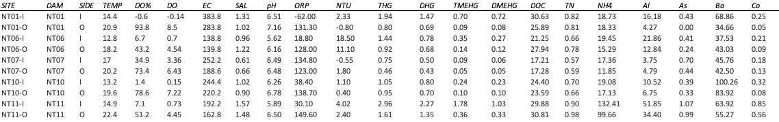
I used boxplots to check the main variables of interest for normality and outliers (Figure 7). Many of the variables are non-normal, positively skewed, and contained outliers. This is typical for water chemistry data, and I was able to check that outliers did not result from an error by comparing total and dissolved concentrations, values yielded from different analytical methods, and relationship analysis.
I also used scatter plots to gain a general understanding of variable relationships (Figure 6.a, 6.b), and to eliminate some trace metal concentrations which have no or weak relationships with other variables (Figure 6.b). 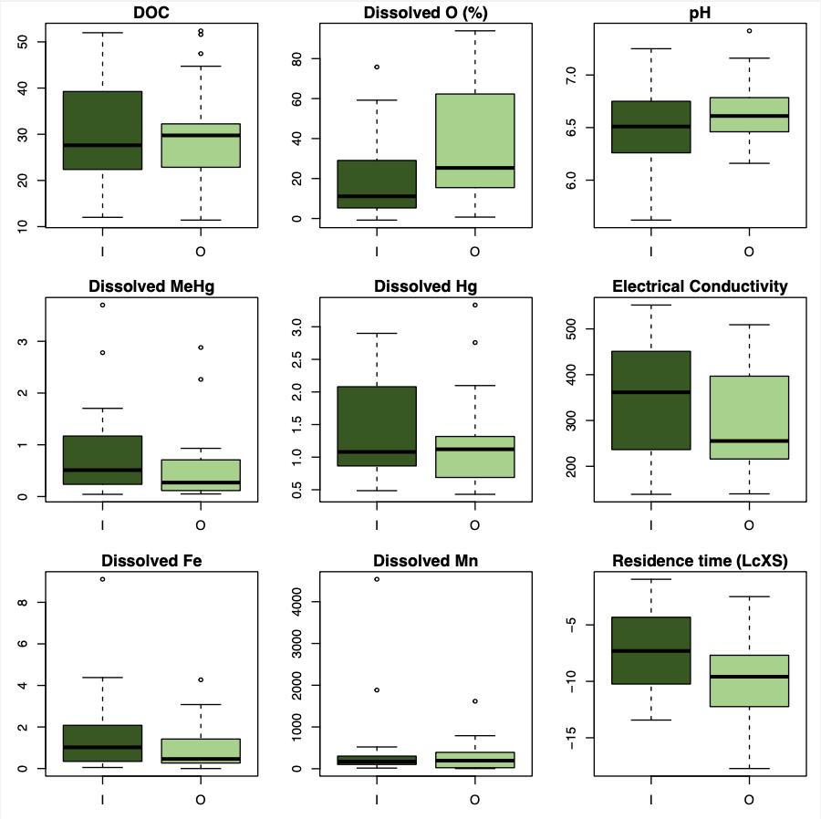
Figure 7. A sample of Boxplots for Inflow (I) and Outflow(O) showing the distribution of the main water chemistry variables of interest to check for normality. Overall, variables appear normal to somewhat positively skewed.
|
Figure 6. A slideshow of figures 6a and 6b:
Figure 6a. Scatterplots showing the relationship between common water chemistry variables. Figure 6.b. A sample of scatterplots showing the relationship between common trace metal concentrations and dissolved oxygen (DO). Metals which showed weak relationships to oxygen, such as Arsenic (As), Barium (Ba) and Molybdenum (Mo), were removed from the dataset prior to analysis |
Relationship exploration
Given outliers and non-normality, I explored the use of NMDS ordination techniques, however the ordination results had high stress values at low dimensions (>0.25), thus yielding suspicious results (Figure 9). Given this constraint, I will present PCAs as they better represent expected and apparent water chemistry relationships in 2 dimensions. I used PCAs to explore the relationship between important variables at the inflow, the outflow, and overall (Figure 8 a-c). The exception is plotting the Inflow and the Outflow data in the same NMDS (Figure 9), where relationships are less clear due to the chemical changes that occur over the pond.
|
Slideshow of Figure 8a-c:
Figure 8.a. PCA of primary water chemistry variables measured at the inflow in August Figure 8.c. PCA of primary water chemistry variables measured at the outflow in August Figure 8.c. PCA of primary water chemistry variables measured in August |
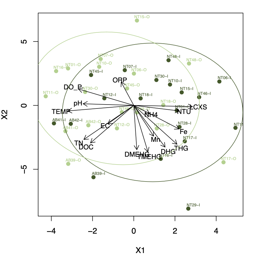
Figure 9. NMDS ordination by standard euclidean distance of primary water chemistry variables measured in August. Ellipses around Inflow and Outflow groups contain 80% of the observations in the ordination.
|
Analysis
I used a one-sided T-test to evaluate the changes in methylmercury concentrations from the inflow to the outflow, running separate tests for June and August samples. This test was run on Dissolved methylmercury because it makes up ~90% of the total methylmercury concentrations both at the inflow and outflow sample points, and is more bioavailable and redox sensitive, and is therefore more sensitive to processed occurring in the pond.
